The efficiency of algorithms is important. Imagine a program that took centuries to calculate the solution to a problem (like Deep Thought from the Hitchhiker’s Guide to the Galaxy), or needed more memory than is available on all the memory chips of all computers in existence. Sounds improbable, but actually if we are not careful about efficiency, our programs can run into these kinds of problems.

When we discuss analysis in the context of algorithms, we are generally referring to their efficiency, or lack of it.

There are two measures of efficiency of we are interested in:

• Time Complexity: the time taken by an algorithm to execute.

• Space Complexity: the amount of memory used by an algorithm while executing.

Time complexity is often considered more important, but space considerations are sometimes relevant too.

The technique for calculating time complexity is to add up how many basic operations an algorithm will execute as a function of the size of its input, and then simplify this expression. Basic operations include things like

• Assignments
• Arithmetic Operations
• Comparison statements
• Calling a function
• Return statements

Take a look at this example. It’s an algorithm that outputs whole numbers from 1 to 100.

n = 100  # Assignment statement
count = 0  # Assignment statement
while count < n:  # Comparison statement
    count += 1  # Arithmetic operation (and assignment!)
    print(count)  # Output statement

One way to count the basic operations is:

n = 100  # Assignment statement 1 time
count = 0  # Assignment statement 1 time
while count < n:  # Comparison statement n times
    count += 1  # Arithmetic operation (and assignment!) n times + n times
    print(count)  # Output statement n times

In total, that's 1 + 1 + n + n + n + n = 4n + 2 basic operations.

Note that there a varying conventions for what constitutes a basic operation, so you will sometimes see the same algorithm analysed differently in terms of its basic operations. However, this is not usually a problem, for reasons which will become clear soon.

What we do now may seem like cheating, but understand that we are interested in how the algorithm perform when the input is very large, since with modern computers small inputs are generally handled extremely fast. This means that as the input size grown, the relevance of all but the most significant term becomes less and less.

In order to determine the complexity of an algorithm, we make some drastic simplifications. Before we get into that though, you need to know what Big-O Notation is.

Big-O notation

In terms of algorithm analysis, Big-O notation is a way of expressing an upper bound on the execution time or space requirements of an algorithm.

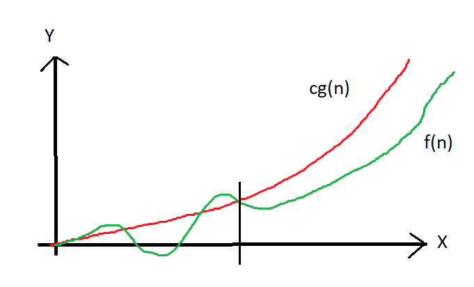
Saying some function f(n) ∈ O(g(n)) means that beyond a certain point, its values are less than some constant multiple of g(n). The notation is read, “f of n is big-o of g of n”. Very often people write = instead of ∈, which although not technically accurate, is generally understood to mean the same thing – “belongs to the class”.

This may look a little scary, if you are not a mathematician. Don’t worry though, it really isn’t that difficult once you understand the basic concept, and much of the mathematical detail can be ignored if all you need is a practical understanding of how the efficiency of different implementations of an algorithm compares.

The reason we are interested in an upper bound is that past a certain point we can be confident that an algorithm won’t perform worse than this bound. This is important as many mission-critical algorithms can’t afford to exceed some worst case scenario, even occasionally.

The common examples of g(n) are:

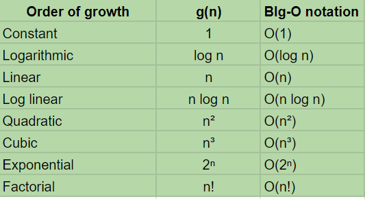
These are listed in descending order of efficiency, with constant (O(1)) being the best and factorial ((O(n!)) being radically inefficient.

How to determine which big-O class an algorithm belongs to

Depending on how we count, an algorithm may look to have, for example, 2n or 5n + 20 basic operations, but for the purposes of analysing the time complexity, we would consider both to be equivalent to O(n).

How so? Well when determining which big-o class an algorithm is in, we

Throw Away Constants

If we have 2n basic operations, we simplify and say the algorithm is O(n) If we have 200 basic operations, we simplify that O(1).

Ignore All But the Largest Term

n + 100 operations is simplified to O(n). So is 500n + 100.

If we have n² + 40n +400 basic operations, we classify the time complexity as O(n²).

Remember, the reason we can make these simplifications is that we are interested in how the number of operations grows as n becomes very large, and the contribution of all but the largest term becomes less significant the larger n becomes.

For practice with this process of simplifying big-o expressions, try expressing the following in the simplest way, as one of the big-o expression is the table above, using the rules just discussed:

• O(n + 10)
• O(100 * n)
• O(50)
• O(n² + n³)
• O(n + n + n + n)

Big-O Notation Summary

To recap, the big idea here is that we want to make an estimate of the number of operations performed by an algorithm in terms of its input size n. We then simplify the resulting expression and categorise the result into one of the big-O classes such as O(n²) (quadratic), O(n) (linear), O(log n) (logarithmic) or O(1) (constant).

This then gives us an upper bound for the time complexity of the algorithm. There may well be situations where the algorithm performs better than this upper bound, but we can say with certainty that it won’t perform worse, assuming n is large enough.

Python Examples of Different Time Complexities

Let’s look at some Python code examples to help to clarify the concept of algorithmic time complexity and big-O notation.

Python Linear Search

In the following example, aside from all the setup code like creating a list of random numbers, the main basic operation is comparison of a list value with a target value. Depending on where in the list the target lies, the algorithm may have to perform up to n comparisons. It may get lucky and exit early, but we use the upper bound and say that this algorithm’s time complexity is O(n). Notice how even with the relatively small (in computing terms) length of the list, there is sometimes a noticeable delay before the result is displayed. Algorithms with O(n) are said to have linear time complexity, which although not terrible, can often be improved upon using alternative approaches.

import random

n = 1000000
target = 2994

data_list = random.sample(range(1, n + 1), n)

for i in range(len(data_list)):
    if data_list[i] == target:
        print("Found at position", i)
        break

Python Binary Search

A great example of an alternative approach producing a drastic improvement in efficiency is the use of Binary Search instead of Linear Search. Binary search reduces the search space by a factor of 2 at each iteration, so instead of having O(n) time complexity, it has O(log n). Since every logarithm can be converted to base 2, the assumption here is that log n means log₂n.

Please note the crucial detail that

For Binary Search to work, the data MUST BE SORTED!

This impacts the time complexity, because sorting the data before applying the algorithm incurs its own cost, depending on the sorting algorithm used.

The binary search algorithm uses an important technique called decrease and conquer. At each stage, half of the data set is discarded, and the algorithm is re-applied to the remaining smaller data set until the search item is found or the exit condition is met.

This halving of the search space is implemented by use of a high pointer and a low pointer (really just position values within the list, rather than actual pointers), and we check the item in the middle of these two pointers to see if it is our search item. If it is, great, we exit, otherwise we move either the high or the low pointer in such as way as to “pincer-in” on our target value. The condition for the while loop ensures that we don’t keep searching for ever.

Here is a simple implantation of Binary Search in Python:

import random

n = 100
max_val = 100
data_list = [random.randint(1, max_val) for i in range(n)]
data_list.sort()
# print(data_list)
# print(len(data_list))
target = 50
lower_bound = 0
upper_bound = len(data_list) - 1
found = False

while not found and lower_bound <= upper_bound:
    mid_point = (lower_bound + upper_bound) // 2
    if data_list[mid_point] == target:
        print("You number has been found at position ", mid_point)
        found = True
    elif data_list[mid_point] < target:
        lower_bound = mid_point + 1
    else:
        upper_bound = mid_point - 1
if not found:
    print("Your number is not in the list.")

Another example of logarithmic time complexity is:

def logarithmic(n):
    val = n
    while val >= 1: 
        val = val // 2
        print(val)  

logarithmic(100)

Output:

50
25
12
6
3
1
0

Note that since we are halving val each time, we approach 0 very quickly (in logarithmic time).

Quadratic Time Complexity

Quadratic time complexity often occurs when nested loops are used, as in the following example:

n = 3
for i in range(n):
    for j in range(n):
        print(f"i: {i}, j: {j}")

Output:

0 0
0 1
0 2
1 0
1 1
1 2
2 0
2 1
2 2

See how for every value of i, there are n values of j? So altogether there are 9 print statements (nxn) when n = 3.

A naïve implementation of an algorithm will often make use of a nested loop, and it is a very common algorithmic problem solving task to design a solution which is more efficient.

Factorial Time Complexity

At the other end of the scale from constant (O(1)) complexity is factorial complexity (O(n!)). This is worse even than exponential complexity (O(2ⁿ)). n! is nx(n-1)x(n-2)x...x2x1, which gets very big very fast. The kinds of algorithms which have factorial time complexity often involve permutations and combinations. For example, finding all the permutations of a collection of items, as in the code below.

Python program for finding permutations

def perms(a_str):
    stack = list(a_str)
    results = [stack.pop()]
    while stack:
        current = stack.pop()
        new_results = []
        for partial in results:
            for i in range(len(partial)+1):
                new_results.append(partial[:i] + current + partial[i:])
        results = new_results
    return results


my_str = "ABCD"
print(perms(my_str))

Time Complexity of Recursive Algorithms

Calculating the time complexity of a recursive algorithm can get a little tricky, but an example will illustrate the basic idea.

Consider the following recursive function:

def count_down(n):
    if n > 0:
        print(n)
        count_down(n-1)

count_down(5)

If we donate its time complexity as T(n) then we can use a recurrence relation to determine its time complexity. The recurrence relation for T(n) is given as:

T(n) = T(n-1) + 1, if n > 0
     = 1 , if n = 0

By using the method of backwards substitution, we can see that

T(n) = T(n-1) + 1 -----------------(1)
T(n-1) = T(n-2) + 1 -----------------(2)
T(n-2) = T(n-3) + 1 -----------------(3)
Substituting (2) in (1), we get
T(n) = T(n-2) + 2 ------------------(4)
Substituting (3) in (4), we get
T(n) = T(n-3) + 3 ------------------(5)
If we continue this for k times, then
T(n) = T(n-k) + k -----------------(6)

Set k = n. Then n - k = 0. We know that T(0) = 1, from the initial recurrence relation.

By substituting the value of k in (6) we get

T(n) = T(n-n) + n
T(n) = T(0) + n
T(n) = 1 + n

For a great explanation of how this works in more detail, you can check out this YouTube video.

Space Complexity

Much of the same reasoning that we apply to time complexity is relevant to space complexity, except that here we are interested in the memory requirements of an algorithm. For example, when considering algorithms which work on arrays, some implementations may use an auxiliary array to store intermediate results, while others may restrict themselves to modifying the original array.

Python Example of O(1) Space Complexity

def my_sum(lst):
    total = 0
    for i in range(len(lst)):
        total += lst[i]
    return total

my_list = [5, 4, 3, 2, 1]
print(my_sum(my_list))

The space complexity of my_sum() is O(1). Why is this? Well, aside from the input, we only have two variables used in the function: total and i. Regardless of the contents of lst we are always only going to have these same two variables, each of which contains a single number. While we add to the total variable, we don’t create or add any new variables. Since we are discussing space not time complexity, we are not interested in the number of operations. So the space complexity is O(1).

Python Example of O(n) Space Complexity

def double(lst):
    new_list = []
    for i in range(len(lst)):
        new_list.append(lst[i] * 2)
    return new_list


my_list = [5, 4, 3, 2, 1]
print(double(my_list))

The space complexity of double() is O(n). Why? Well, the longer the list passed to the function is, the longer the new list that gets returned is. This means that the function’s required space will increase depending on the length of the input list. Hence the space requirement increases as the size of the input list increases, so the function has O(n) space complexity.

More Detail on Asymptotic Complexity

Other measures than big-O are used for measuring the space and time complexity of algorithms. However the topic can get quite complex, and for general usage, sticking with big-O is often sufficient. There is also some discrepancy in usage between programmers and mathematicians. For example, it is often technically more appropriate to use Θ(), which represents a tight bound as opposed to the upper bound given by big-O, but since the upper bound is still technically correct, the difference is often ignored.

For those interested in a bit more detail, the image at the top of this post represents the following formal definition of big-O notation:

f(n) = O(g(n)) means there are positive constants c and k, such that 0 ≤ f(n) ≤ cg(n) for all n ≥ k. The values of c and k must be fixed for the function f and must not depend on n.

Conclusion

This article has gone into detail about how to analyse the time and space complexity of algorithms, with many examples in Python code. I hope you have found it interesting and useful. For a related article which shows how to explore the time complexity of Python algorithms by plotting the graph of their execution times, see Time Complexity in Python Programming.

Happy computing!

Sharing is caring!