This is an article about time complexity in Python programming. In it we explore what is meant by time complexity and show how the same program can be dramatically more or less efficient in terms of execution time depending on the algorithm used.

Topics covered:

• What is time complexity in Python programming?
• “Big O” notation
• Plotting graphs of time complexity with pyplot

Time complexity is a topic which many self-taught programmers who have not studied Computer Science tend to shy away from. However it is well worth the effort to learn at least the basics of this topic as it will empower you to write much more efficient code.

The subject of Time Complexity in programming can seem a little daunting at first with some unfamiliar mathematical notation and the various graphs which are used to express how the time taken for an algorithm to complete grows as the size of its input grows.

However:

The basic concept of time complexity is simple: looking a graph of execution time on the y-axis plotted against input size on the x-axis, we want to keep the height of the y values as low as possible as we move along the x-axis.

You can get a good intuitive understanding of time complexity by studying the graphs of various mathematical functions and how the height of the graph grows as we move along the x-axis. The graph below shows how various types of mathematical function behave. The idea is that the execution time of algorithms can be seen to grow in a similar fashion to one of these types function, depending on its implementation. Our goal is to write algorithms which behave like the slower growing functions and avoid implementations which behave like the rapidly growing ones.

There is a lot of detail that you can go into about whether we are considering the best-case, worst-case, average-case etc, but that is often more detail than you need. To keep it simple, lets just say:

• exponential: very bad
• cubic: bad, avoid if possible
• quadratic: bad, avoid if possible
• linear: good
• logarithmic: great
• constant: you hit the jackpot

Big O notation is a way to refer to these types of growth.

• O(2ⁿ): exponential
• O(n³): cubic
• O(n²): quadratic
• O(n): linear
• O(log n): logarithmic
• O(1): constant

Recommended Books for Learning Algorithms and Data Structures

Please note, as an Amazon Associate I earn from qualifying purchases.

For the remainder of this article, rather than focusing on the general theory of time complexity, we will be looking at a specific algorithm that counts the common elements in a list.

Take a look at this graph:

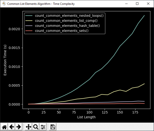
You can clearly see on the graph how the execution time of count_common_elements_nested_loops() grows much more rapidly than for count_common_elements_sets()

it makes use of pyplot from matplotlib, a powerful plotting library for Python. The details of how to use pyplot are for another article, but by examining the code below you can get a sense of how it works. The code uses perf_counter from the time library to calculate the execution time of different algorithms to perform the task of counting common elements is a list. You can see from the resulting graph that there is a significant difference between the implementations in terms of time complexity as the size of the input to each function grows..

Time Complexity Example Python Code Listing

import random
import time
import matplotlib.pyplot as plt

MAX_LEN = 200  # Maximum length of input list.


def count_common_elements_nested_loops(l1, l2):
    common_elements = []
    count = 0
    for v in l1:
        for w in l2:
            if w == v:
                common_elements.append(w)
                count += 1
    return count


def count_common_elements_list_comp(l1, l2):
    common_elements = [x for x in l1 if x in l2]
    return len(common_elements)


def count_common_elements_sets(l1, l2):
    common_elements = set(l1).intersection(l2)
    return len(common_elements)


def count_common_elements_hash_table(l1, l2):
    table = {}
    common_elements = []
    for v in l1:
        table[v] = True
    count = 0
    for w in l2:
        if table.get(w):  # Avoid KeyError that would arise with table[w]
            common_elements.append(w)
            count += 1
    return count


if __name__ == "__main__":

    # Initialise results containers
    lengths_nested = []
    times_nested = []
    lengths_comp = []
    times_comp = []
    lengths_hash_table = []
    times_hash_table = []
    lengths_sets = []
    times_sets = []

    for length in range(0, MAX_LEN, 10):
        # Generate random lists
        l1 = [random.randint(0, 99) for _ in range(length)]
        l2 = [random.randint(0, 99) for _ in range(length)]

        # Time execution for nested lists version
        start = time.perf_counter()
        count_common_elements_nested_loops(l1, l2)
        end = time.perf_counter()

        # Store results
        lengths_nested.append(length)
        times_nested.append(end - start)

        # Time execution for list comprehension version
        start = time.perf_counter()
        count_common_elements_list_comp(l1, l2)
        end = time.perf_counter()

        # Store results
        lengths_comp.append(length)
        times_comp.append(end - start)

        # Time execution for hash table version
        start = time.perf_counter()
        count_common_elements_hash_table(l1, l2)
        end = time.perf_counter()

        # Store results
        lengths_hash_table.append(length)
        times_hash_table.append(end - start)

        # Time execution for sets version
        start = time.perf_counter()
        count_common_elements_sets(l1, l2)
        end = time.perf_counter()

        # Store results
        lengths_sets.append(length)
        times_sets.append(end - start)

    # Plot results
    plt.style.use("dark_background")
    plt.figure().canvas.manager.set_window_title("Common List Elements Algorithm - Time Complexity")
    plt.xlabel("List Length")
    plt.ylabel("Execution Time (s)")
    plt.plot(lengths_nested, times_nested, label="count_common_elements_nested_loops()")
    plt.plot(lengths_comp, times_comp, label="count_common_elements_list_comp()")
    plt.plot(lengths_hash_table, times_hash_table, label="count_common_elements_hash_table()")
    plt.plot(lengths_sets, times_sets, label="count_common_elements_sets()")
    plt.legend()
    plt.tight_layout()
    plt.show()

Some observations:

• The difference in performance is striking, particularly with the speed of growth of the nested for loops version…
• You might expect list comprehensions to have similar time complexity to nested for loops, since list comprehensions can be created with nested for loops. However, the implementation of list comprehensions “under the hood” is much more efficient.
• The same applies for sets vs hash_tables, since sets make use of hash_tables. However, The set.intersection method implemented in C. it’s worth remembering that many Built-in functions / methods will almost always be faster than equivalent algorithms that get executed at the python interpreter level.

This article was meant to give you a practical experience of working with time complexity in Python as an introduction to the topic. Time complexity is a big subject and there are many resource available to help you learn online. One place you can get practice is on sites such as hackerrank and project euler, where the “brute force” appraoch may provide correct answers, but not in the required time-frame.

Happy computing!

Sharing is caring!