I’ve been enjoying reading A Programmer’s Introduction to Mathematics by Jeremy Kun recently. After the introduction, the first main topic it covers is a neat trick for sharing secrets (encrypting messages) so that they can be decoded using polynomial functions.

Being a firm believer in learning by doing, I immediately got stuck in and started exploring. It has been some time since I worked much with polynomials, so to get a feel for what I was doing, I wrote a Python program to help me visualise polynomial functions with given coefficients. That is what I want to share in this blog post.

A polynomial function is a function such as a quadratic, a cubic, a quartic, and so on, involving only non-negative integer powers of its input variable.

The form of a polynomial is

where the a’s are real numbers (called the coefficients of the polynomial). For example:

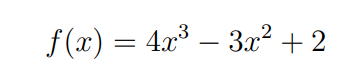
is a polynomial of degree 3, as 3 is the highest power of x in the formula. This is called a cubic polynomial. Notice that we don’t need every power of x up to 3: we only need to know the highest power of x to find out the degree.

Python Code Listing for Plotting Polynomials

This program uses matplotlib for plotting and numpy for easy array manipulation, so you will have to install these packages if you haven’t already. The code is commented to help you understand how it works.

import numpy as np
import matplotlib.pyplot as plt

plt.style.use("fivethirtyeight")


def polynomial_coefficients(xs, coeffs):
    """ Returns a list of function outputs (`ys`) for a polynomial with the given coefficients and
    a list of input values (`xs`).

    The coefficients must go in order from a0 to an, and all must be included, even if the value is 0.
    """
    order = len(coeffs)
    print(f'# This is a polynomial of order {order - 1}.')

    ys = np.zeros(len(xs))  # Initialise an array of zeros of the required length.
    for i in range(order):
        ys += coeffs[i] * xs ** i
    return ys


xs = np.linspace(0, 9, 10)  # Change this range according to your needs. Start, stop, number of steps.
coeffs = [0, 0, 1]  # x^2

# xs = np.linspace(-5, 5, 100)  # Change this range according to your needs. Start, stop, number of steps.
# coeffs = [2, 0, -3, 4]  # 4*x^3 - 3*x^2 + 2

plt.gcf().canvas.set_window_title('Fun with Polynomials')  # Set window title
plt.plot(xs, polynomial_coefficients(xs, coeffs))
plt.axhline(y=0, color='r')  # Show xs axis
plt.axvline(x=0, color='r')  # Show y axis
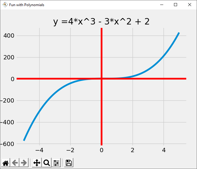
plt.title("y =4*x^3 - 3*x^2 + 2")  # Set plot title
plt.show()

There are a couple of example polynomials provided in the code. Once you have checked out a simple quadratic (y = x^2) using the two lines below:

xs = np.linspace(0, 9, 10)
coeffs = [0, 0, 1]  # x^2

you can uncomment these two lines, then once you have the hang of how the program works, you can try your setting up and plotting your own polynomials:

# xs = np.linspace(-5, 5, 100)  # Change this range according to your needs. Start, stop, number of steps.
# coeffs = [2, 0, -3, 4]  # 4*x^3 - 3*x^2 + 2

A Programmer’s Introduction to Mathematics: Second Edition by Jeremy Kun

I thoroughly recommend this book for anyone keen to explore the relationship between Mathematics and Programming at a roughly undergraduate level. It is friendly and thorough, and there is a full repository of Python code examples available on GitHub.

As an Amazon Associate I earn from qualifying purchases.

This post has explored how to plot polynomials with Python and matplotlib. I hope you found it interesting and helpful. Happy computing!

Sharing is caring!