The ability to make sense of data is more important than ever in today’s complex world. Data is everywhere, and being able to interpret it empowers us to make effective decisions, as well as to avoid being misled when it is presented in misleading ways, whether intentionally or not.

Some of the areas where understanding of data analysis techniques is essential are:

• Medicine
• Business
• Government
• Humanitarian Aid
• Many branches of science
• Artificial Intelligence/Machine Learning

The Python programming language is a perfect tool for analysing and working with data. There are many powerful open source libraries available which enable us to focus on the the task at hand rather than getting bogged down in implementation details. Two of the most powerful and popular libraries for working with data in Python are pandas and matplotlib.

Python Pandas Module

Pandas is a powerful and easy to use open source data analysis and manipulation tool, built on top of the Python programming language. The name is derived from the term “panel data analysis”, a statistical method used in areas such as social science, epidemiology, and econometrics.

Pandas uses Series and DataFrame data structures to represent data in a way that is suitable for analysis. There are also methods for convenient data filtering. One powerful feature is the ability to read data from a variety of formats including directly from an online source.

Matplotlib

Matplotlib is an awesome Python library for producing detailed and attractive visualizations in Python. You will soon discover how easily it is to create plots of your data with many customisation options.

Let’s get started!

If you don’t already have them, you will need to install the packages first. The way you do this will depend on your situation. One of the common ways is to use pip from a terminal.

• pip install pandas
• pip install matplotlib

Installing packages is an essential skill for anyone wishing to use more than just the basic functionality of Python. There are thousands of amazing packages available. You can read more about how to install Python packages here.

For the purposes of this lesson we are going to use tiny dataset about some trials for antidepressants. The dataset comes from the DASL website. I have chosen this dataset because it is “real world” meaning the data was collected from real experiments. Please bear in mind though that the data set it small and there is insufficient information provided with it to draw any far-reaching conclusions.

The dataset is shown below for reference.

Study   Treated Placebo
Blashki.et.al.  1.75    1.02
Byerly.et.al.   2.3 1.37
Claghorn.et.al. 1.91    1.49
Davidson&Turnbull   4.77    2.28
Elkin.et.al.    2.35    2.01
Goldberg.et.al. 0.44    0.44
Joffe.et.al.    1.43    0.61
Kahn.et.al. 2.25    1.48
Kiev&Okerson    0.44    0.42
Lydiard 2.59    1.93
Ravaris.et.al.  1.42    0.91
Rickels.et.al.  1.86    1.45
Rickels&Case    1.71    1.17
Robinson.et.al. 1.13    0.76
Schweizer.et.al.    3.13    2.13
Stark&Hardison  1.4 1.03
van.der.Velde   0.66    0.1
White.et.al.    1.5 1.14
Zung    0.88    0.95

If you look at the website where this data comes from, you will see the following story (as an aside, it’s worth considering that one of the main goals of data analysis is to find the story behind the data.)

Story: A study compared the effectiveness of several antidepressants by examining the experiments in which they had passed the FDA requirements. Each of those experiments compared the active drug with a placebo, an inert pill given to some of the subjects. In each experiment some patients treated with the placebo had improved, a phenomenon called the placebo effect. Patients’ depression levels were evaluated on the Hamilton Depression Rating Scale, where larger numbers indicate greater improvement. (The Hamilton scale is a widely accepted standard that was used in each of the independently run studies.) It is well-understood that placebos can have a strong therapeutic effect on depression, but separating the placebo effect from the medical effect can be difficult.

One thing to always keep in mind when working with data is exactly what the data represents!

In this example, there is not a lot of information on exactly what each data point represents. I’m going to assume that each value given for the Hamilton Depression Rating Scale for each study represents an average (don’t forget this term is ambiguous – let’s assume the mean) value for each sample in the study.

Here’s some Python code we can use to get some descriptive statistics for the data set. Notice how easy it is to read in data using pandas, even from a remote URL. If you want to download the data and load it from a local file, use the commented line instead.

import pandas as pd
import matplotlib.pyplot as plt


df = pd.read_csv("https://dasl.datadescription.com/download/data/3054", sep="\t")
# df = pd.read_csv("antidepressants.txt", sep="\t")
print(df.describe())

The output from the above code is

         Treated    Placebo
count  19.000000  19.000000
mean    1.785263   1.194211
std     1.022428   0.606615
min     0.440000   0.100000
25%     1.265000   0.835000
50%     1.710000   1.140000
75%     2.275000   1.485000
max     4.770000   2.280000

Depending on your level of experience with data analysis, these values will make more or less sense to you. What they represent is a basic description of the dataset in terms of its size, mean value and the distribution of the the data. The % figures are for the quartiles which break the data into four sections to help us to understand how “spread out” the data is.

Looking at the numeric data, we can start to make some tentative inferences. For example, the treated patients have a mean score 0.6 higher than for the placebo group. This suggests that the treatment may be more effective than the placebo, but more information is needed to be confident as to whether this is actually true, and to what degree.

Python Pandas DataFrame Objects

In terms of the Python code above, them main thing to note is that we are importing the libraries we need, and then creating a DataFrame object (df in our code), which contains our data and has many useful properties and methods we can use to explore it.

For example, if you add print(df.head) to your existing code, you will get the following output:

               Study  Treated  Placebo
0     Blashki.et.al.     1.75     1.02
1      Byerly.et.al.     2.30     1.37
2    Claghorn.et.al.     1.91     1.49
3  Davidson&Turnbull     4.77     2.28
4       Elkin.et.al.     2.35     2.01

You can see the the data has been structured with a numerical index and three columns which we can refer to by name to reference particular data points.

Exploring a dataset using Python and Matplotlib – Scatterplot

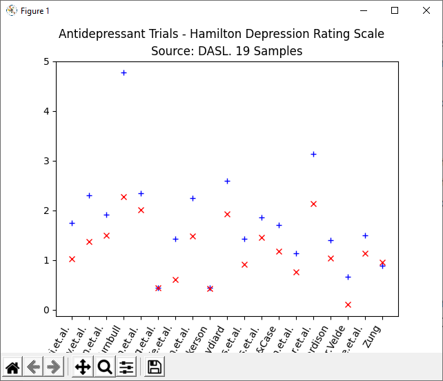
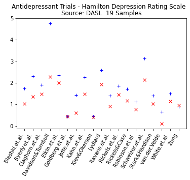
To get a clearer picture (literally) of the data, we can use Python’s matplotlib library to create many different visual representations. Add the code below to your existing code from above to produce a simple plot of the data, using + and x to mark values on the y-axis.

treated = df.Treated
placebo = df.Placebo
study = df.Study
plt.suptitle("Antidepressant Trials - Hamilton Depression Rating Scale")
plt.title("Source: DASL. 19 Samples")
plt.plot(study, treated, "+", color="blue")
plt.plot(placebo, "x", color="red" )
plt.xticks(rotation=60, ha="right")
plt.show()

The syntax is very intuitive. The main things to note are that we have extracted the individual columns from the dataframe and used them as arguments in plt.plot(). There are also a few details relating to display parameters, but these are mostly self-explanatory.

Exploring a dataset using Python and Matplotlib – Box and Whiskers Plots

A scatterplot is a great way to get a visual overview of a dataset, but it makes reading precise values difficult. Another common tool to represent data visually is a box and whiskers plot. This contains more or less the same information as we gleaned above using df.describe(), but in an easily digestible visual format.

Add the following code to what you have already:

labels = ["Treated", "Placebo"]
data = [treated, placebo]
plt.boxplot(data, vert=False, patch_artist=True, labels=labels, showfliers=False)
plt.suptitle("Antidepressant Trials - Hamilton Depression Rating Scale")
plt.title("Source: DASL. 19 Samples")
plt.show()

and you will get this figure.

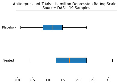
This makes comparison of the values from the treated groups with the placebo groups easier to perform. You can immediately see the relative positions of the mean values, but you can also see that the spread for the treated groups is wider than for the placebo groups. In a future article we will look in more detail at how these kinds of details affect the kinds of inferences which can be made when comparing datasets. For example we will see how to add error bars to our plots.

For now though there is plenty to get your teeth into with what we have explored so far. Once you have tried out everything we have covered for yourself, don’t stop there – that is just the beginning. Try using the techniques we have discussed on different datasets and seeing what kinds of conclusions you can draw from the various representations that Python makes available to you with just a few lines of code. See what story you can tell from the data. There is a great selection of datasets available from the same place I got the antidepressant trial data used in this article – DASL – The Data And Story Library.

This lesson has covered some important fundamental concepts in data literacy and introduces some powerful Python tools you can use to explore and represent data – the pandas and matplotlib libraries. I hope you have found the lesson useful.

Happy computing!

Sharing is caring!