Computer programmers in general spend a fair bit of time engaged in algorithmic thinking. The idea of metacognition is basically “thinking about thinking”, with an implied agenda of improving our thinking. It stands to reason then that metacognition could be of use to programmers, as it provides the opportunity to improve our algorithmic thinking.
However, it doesn’t stop there. Once we become interested in thinking about thinking, a whole world of possibilities opens up, and if are open to the possibility that our thinking could be improved, then great things are possible. Programmers are probably better placed than many to recognise the need for improvement in our thinking, as we are generally in the habit of learning new things on a very regular basis. After all, we would not get far as developers if we weren’t comfortable with the idea that we don’t already know everything. This is perhaps a less common attitude outside of the programming world.
There had been a great deal of work done in the area of metacognition. Much of the foundational work was done by Edward de Bono. He has authored many books and designed courses of learning and tools which are in widespread use in many institutions around the world. I like to think of him as “the Grandfather of Metacognition”, but to be fair I don’t know enough about his influences to know whether this is a deserved title.
A common issue with de Bono’s work is that people coming across it often fail to recognise its significance and power. Many of the ideas are so simple that they are often dismissed as trivial. There is also the cultural trait of intelligent people often not recognizing the need to improve their thinking. If de Bono’s work is something which interests you, you will have to judge its value for yourself. In my personal opinion, it is nothing short of revolutionary, in that it is the biggest step forward in human reasoning since the time of the great Greek philosophers such as Plato and Aristotle.
Directional Idea Maps with Python
So what does this have to do with Python programming?
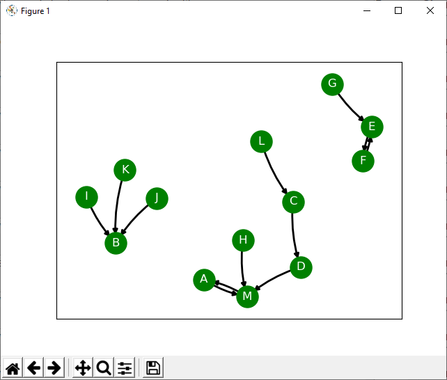
I want to share with you a metacognitive tool written in Python for exploring the relationship between elements in a situation. It is inspired by Edward de Bono’s flowscapes. You can get the code from my GitHub account. The way the tool works is that it creates a directed graph where the nodes represent different aspects of the situation under consideration.
Once a graph is created, it gives us a visual representation of the connections between elements. There is no one correct interpretation of the resulting graph, but instead you will notice certain features such as loops and gravity wells which may give you unexpected insight into the situation you are exploring.
Usage:
- List the elements present in the situation you want to explore
- For each element, choose just one element it flows most naturally towards, based on any definition of “flow towards” you like.
- Hit submit and see a visual representation of the relationship between the elements
- Interpret at will
- You can save/load previous sessions if required.
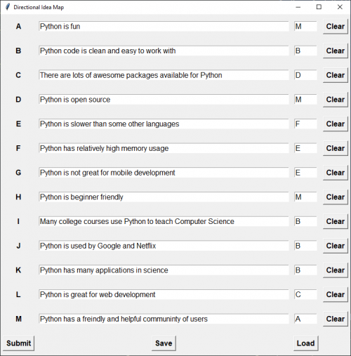
The application can save and load previous sessions in json format for future use. Note that you have to produce a graph by clicking Submit before you can save a session. Also note that there are some validation rules which mean you won’t be able to submit your form under certain conditions (e.g. one node flowing to multiple other nodes).
Python Code for the Idea Maps Metacognitive Tool
I have provided the Python code for this application below for reference. A couple of things to note are:
TkinterandMatplotlibdo not play nicely together. For this fairly simple application, I didn’t need to usematplotlib.backends.backend_tkaggbut for anything more complex, you will need to explore that approach to working with both libraries together. You can see an example here.- The
networkxpackage (which you will need to install usingpip) needed a slight modification to position the nodes correctly when the graphs is not connected. That is what themy_reingold.pyfiles is for, and it overrides the originalnetworkxversion.
# idea_maps.py

import matplotlib.pyplot as plt
import json
import tkinter as tk
from tkinter import filedialog
import networkx as nx
from my_reingold import my_reingold
nx.drawing.layout._fruchterman_reingold = my_reingold


NUM_ROWS = 13
BOLD_FONT = ("calbri", 12, "bold")
NORMAL_FONT = ("calbri", 12, "normal")


def create_widgets():
    for i in range(NUM_ROWS):
        key = chr(i + 65)
        this_row = widgets[key] = {}
        this_row["label"] = tk.Label(root, text=key, font=BOLD_FONT)
        this_row["label"].grid(row=i, column=0, padx=5, pady=10)
        this_row["factor_field"] = tk.Entry(root, width=60, font=NORMAL_FONT)
        this_row["factor_field"].grid(row=i, column=1, padx=5, pady=10)
        this_row["target_node_field"] = tk.Entry(
            root, width=5, font=NORMAL_FONT)
        this_row["target_node_field"].grid(row=i, column=2, padx=5, pady=10)
        this_row["clear_button"] = tk.Button(root, text="Clear", command=lambda key=key: clear(
            key), font=BOLD_FONT).grid(row=i, column=3, padx=5, pady=10)

    submit_button = tk.Button(root, text="Submit", command=submit,
                              font=BOLD_FONT).grid(row=NUM_ROWS + 1, column=0, padx=5, pady=10)
    save_button = tk.Button(root, text="Save", command=save,
                            font=BOLD_FONT).grid(row=NUM_ROWS + 1, column=1, padx=5, pady=10)
    load_button = tk.Button(root, text="Load", command=load,
                            font=BOLD_FONT).grid(row=NUM_ROWS + 1, column=2, padx=5, pady=10)


def validate_fields():
    legal_targets = list(widgets.keys()) + [""]  # to allow empty fields

    for key, row in widgets.items():
        factor_field_contents = row["factor_field"].get()
        target_node_field_contents = row["target_node_field"].get().upper()

        # Every target must belong to the set of available factors
        if target_node_field_contents not in legal_targets:
            return False

        #  Target factor field must not be empty
        if target_node_field_contents:
            if not widgets[target_node_field_contents]["factor_field"].get():
                return False

        # Every non-empty factor must have a target
        flen0 = len(factor_field_contents) == 0
        tlen0 = len(target_node_field_contents) == 0
        if (flen0 and not tlen0) or (not flen0 and tlen0):
            return False

    return True


def submit():
    plt.close()
    if validate_fields():
        G = nx.DiGraph()
        edges = []
        for key, row in widgets.items():
            factor_field_contents = row["factor_field"].get()
            target_node_field_contents = row["target_node_field"].get().upper()
            if factor_field_contents != "" and target_node_field_contents != "":
                edges.append((key, target_node_field_contents))
                data[key] = {"factor": factor_field_contents,
                             "target_node": target_node_field_contents}
        G.add_edges_from(edges)
        # pos = nx.spring_layout(G, k=1.0, iterations=50)
        pos = nx.spring_layout(G)
        nx.draw_networkx_nodes(G, pos, node_size=500, node_color="green")
        nx.draw_networkx_labels(G, pos, font_color="white")
        nx.draw_networkx_edges(
            G, pos, connectionstyle='arc3, rad = 0.1', width=2, arrows=True)
        plt.show()


def save():
    print("Attempting to save.")
    # print(f"data: {data}")
    if data:
        try:
            filename = filedialog.asksaveasfile(mode='w')
            json_data = json.dumps(data, indent=4)
            filename.write(json_data)
            print("Data saved.")
        except OSError as e:
            print(e)


def load():
    for key, entries in widgets.items():
        entries["factor_field"].delete(0, "end")
        entries["target_node_field"].delete(0, "end")
    try:
        filename = filedialog.askopenfile(mode='r')
        loaded_data = json.loads(filename.read())
        # print(loaded_data)
        for key, entries in loaded_data.items():
            widgets[key]["factor_field"].insert(0, entries["factor"])
            widgets[key]["target_node_field"].insert(0, entries["target_node"])
    except OSError as e:
        print(e)


def clear(key):
    widgets[key]["factor_field"].delete(0, "end")
    widgets[key]["target_node_field"].delete(0, "end")


if __name__ == "__main__":
    data = {}
    widgets = {}
    root = tk.Tk()
    root.title("Directional Idea Map")
    create_widgets()
    root.mainloop()
# my_reingold.py

def my_reingold(
    A, k=None, pos=None, fixed=None, iterations=50, threshold=1e-4, dim=2, seed=None
):
    # Position nodes in adjacency matrix A using Fruchterman-Reingold
    # Entry point for NetworkX graph is fruchterman_reingold_layout()
    import numpy as np

    try:
        nnodes, _ = A.shape
    except AttributeError as e:
        msg = "fruchterman_reingold() takes an adjacency matrix as input"
        raise nx.NetworkXError(msg) from e

    if pos is None:
        # random initial positions
        pos = np.asarray(seed.rand(nnodes, dim), dtype=A.dtype)
    else:
        # make sure positions are of same type as matrix
        pos = pos.astype(A.dtype)

    # optimal distance between nodes
    if k is None:
        k = np.sqrt(1.0 / nnodes)
    # the initial "temperature"  is about .1 of domain area (=1x1)
    # this is the largest step allowed in the dynamics.
    # We need to calculate this in case our fixed positions force our domain
    # to be much bigger than 1x1
    t = max(max(pos.T[0]) - min(pos.T[0]), max(pos.T[1]) - min(pos.T[1])) * 0.1
    # simple cooling scheme.
    # linearly step down by dt on each iteration so last iteration is size dt.
    dt = t / float(iterations + 1)
    delta = np.zeros((pos.shape[0], pos.shape[0], pos.shape[1]), dtype=A.dtype)
    # the inscrutable (but fast) version
    # this is still O(V^2)
    # could use multilevel methods to speed this up significantly
    for iteration in range(iterations):
        # matrix of difference between points
        delta = pos[:, np.newaxis, :] - pos[np.newaxis, :, :]
        # distance between points
        distance = np.linalg.norm(delta, axis=-1)
        # enforce minimum distance of 0.01
        np.clip(distance, 0.01, None, out=distance)
        # displacement "force"
        displacement = np.einsum(
            "ijk,ij->ik", delta, (k * k / distance ** 2 - A * distance / k)
        )
        ### Source code modified by RA
        # Prevent things from flying off into infinity if not connected
        displacement = displacement - pos / ( k * np.sqrt(nnodes))
        ### END of modifications
        # update positions
        length = np.linalg.norm(displacement, axis=-1)
        length = np.where(length < 0.01, 0.1, length)
        delta_pos = np.einsum("ij,i->ij", displacement, t / length)
        if fixed is not None:
            # don't change positions of fixed nodes
            delta_pos[fixed] = 0.0
        pos += delta_pos
        # cool temperature
        t -= dt
        err = np.linalg.norm(delta_pos) / nnodes
        if err < threshold:
            break
    return pos
I hope you find this application interesting and helpful.
Happy computing and cogitating.