
In this article we are going to explore probability with Python with particular emphasis on discrete random variables.
Discrete values are ones which can be counted as opposed to measured. This is a fundamental distinction in mathematics. Something that not everyone realises about measurements is that they can never be fully accurate. For example, if I tell you that a person’s height is 1.77m, that value has been rounded to two decimal places. If I were to measure more precisely, the height might turn out to be 1.77132m to five decimal places. This is quite precise, but in theory the precision could be improved ad infinitum.
This is not the case with discrete values. They always represent an exact number. This means in some ways they are easier to work with.
Discrete Random Variables
A discrete random variable is a variable which only takes discrete values, determined by the outcome of some random phenomenon. Discrete random variable are often denoted by a capital letter (E.g. X, Y, Z). The probability of each value of a discrete random variable occurring is between 0 and 1, and the sum of all the probabilities is equal to 1.
Some examples of discrete random variables are:
- Outcome of flipping a coin
- Outcome of rolling a die
- Number of occupants of a household
- number of students in a class
- Marks in an exam
- The number of applicants for a job.
Discrete Probability Distributions
A random variable can take different values at different times. In many situations, some values will be encountered more often than others. The description of the probability of each possible value that a discrete random variable can take is called a discrete probability distribution. The technical name for the function mapping a particular value of a discrete random variable to it’s associated probability is a probability mass function (pmf).
Confused by all the terminology? Don’t worry. We’ll take a look at some examples now, and use Python to help us understand discrete probability distributions.
Python Code Listing for a Discrete Probability Distribution
Check out this example. You may need to install some of the modules if you haven’t already. If you are not familiar with Numpy, Matplotlib and Seaborn, allow me to introduce you…
import numpy as np
import matplotlib.pyplot as plt
import seaborn as sns

NUM_ROLLS = 1000

values = [1, 2, 3, 4, 5, 6]
sample = np.random.choice(values, NUM_ROLLS)

# Numpy arrays containing counts for each side
side, count = np.unique(sample, return_counts=True)
probs = count / len(sample)

# Plot the results
sns.barplot(side, probs)
plt.title(
    f"Discrete Probability Distribution for Fair 6-Sided Die ({NUM_ROLLS} rolls)")
plt.ylabel("Probability")
plt.xlabel("Outcome")
plt.show()
In this example there is an implied random variable (let’s call it X), which can take the values 1, 2, 3, 4, 5 or 6. A sample of NUM_ROLL size is generated and the results plotted using seaborn and matplotlib.
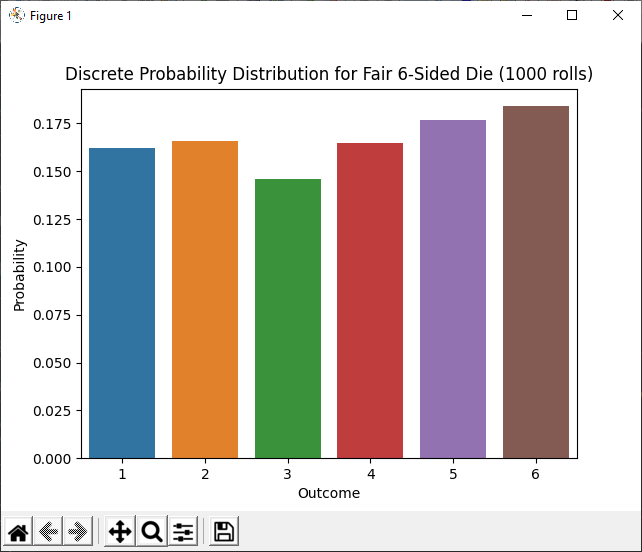
The code makes use of numpy to create a sample, and seaborn to easily create a visually clear and pleasing bar plot.
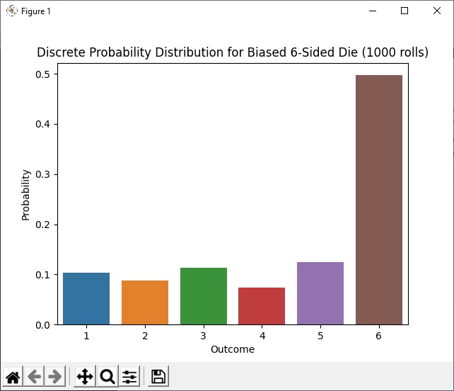
Simulating a Biased Die with Python
The code above can be amended just slightly to produce and display a sample for a weighted (biased) die. Here the 6 side has a probability of 0.5 while for all the other sides it is 0.1.
import numpy as np
import matplotlib.pyplot as plt
import seaborn as sns

NUM_ROLLS = 1000

values = [1, 2, 3, 4, 5, 6]
probs = [0.1, 0.1, 0.1, 0.1, 0.1, 0.5]

# Draw a weighted sample
sample = np.random.choice(values, NUM_ROLLS, p=probs)

# Numpy arrays containing counts for each side
side, count = np.unique(sample, return_counts=True)
probs = count / len(sample)

# Plot the results
sns.barplot(side, probs)
plt.title(
    f"Discrete Probability Distribution for Biased 6-Sided Die ({NUM_ROLLS} rolls)")
plt.ylabel("Probability")
plt.xlabel("Outcome")
plt.show()
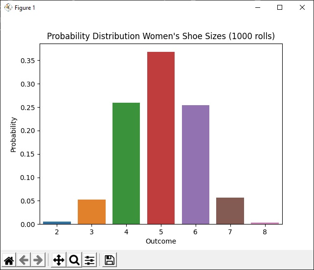
Discrete Normal Distribution of Shoe Sizes with Python
Finally, let’s take a look at how we can create a normal distribution and plot it using Python, Numpy and Seaborn.
Lets say that we learn women’s shoes in a particular population have a mean size of 5 with a standard deviation of 1. We can use the same code as before to plot the distribution, except that we create our sample with the following two lines instead of sample = np.random.choice(values, NUM_ROLLS, p=probs):
sample = np.random.normal(loc=5, scale=1, size=NUM_ROLLS)
sample = np.round(sample).astype(int)  # Convert to integers
Here is the result – a discreet normal distribution for women’s shoe sizes:
In this article we have looked how to create and plot discrete probability distributions with Python. I hope you found it interesting and useful.
Happy computing!